Introduction
The crestr package has been designed for two independent
but complementary modelling purposes [1]. The
probabilistic proxy-climate responses can be used to quantitatively
reconstruct climate from their statistical combination [2-3], or they can be
used in a more quantitative way to determine the (relative) climate
sensitivities of different taxa in a given area to characterise past
ecological changes [4-5].
In both cases, the difficulty of running a CREST analysis lies in the definition of the study-specific parameters of the algorithm, which can make the learning curve a bit steep at the beginning. However, default values are provided for all parameters to enable an easy and rapid generation of preliminary results that users can then use as a reasonable first estimate before adapting the model to their data. To guide users in this task and avoid the standard ‘black box’ criticism faced by many complex statistical tools, a large array of publication-ready, graphical diagnostic tools was designed to represent CREST data in a standardised way automatically. These tools include plots of the calibration data, the estimated climate responses, the reconstructions and many more. They can be used to look at the data from different perspectives to help understand why the results are what they are and possibly help identify potential issues or biases in the selected data and parameters. Such diagnostic tools are available for every step of the process, and, as exemplified by this example, they can be generated with a single line of R code.
This introductory tutorial presents the most important steps of a CREST reconstruction using pseudo-data. The different modelling assumptions are illustrated using the various graphical diagnostic tools proposed by the package. In the first part, the pseudo-data and their different characteristics are presented, the second part describes how to access the pseudo-data from crestr and in the last part, the data are used to reconstruct both temperature and precipitation. The R code used in this last part can be accessed here.
Description of the pseudo-data
This example reconstructs temperature and precipitation from six taxa with different sensitivities to the observed climate gradients. For simplicity, the temperature data are constructed as an East-West climate gradient, while the precipitation data are designed as a North-South gradient. This results in, for instance, cold and rainy conditions in the bottom-left corner and warm and dry conditions in the opposite, top right corner (see Fig. 1). Such gradients are unrealistic, but they explain different concepts, such as the sensitivity of taxa to one or both variables.
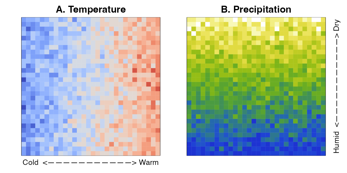
Fig. 1: Randomly generated temperature (A) and precipitation (B) climate data.
In this environment, six different pseudo-species have been created, each one with specific climate preferences (Fig. 2):
- Taxon1 is adapted to hot and dry conditions.
- Taxon2 is adapted to hot conditions and tolerates a large range of rainfall values.
- Taxon3 is adapted to cold conditions and tolerates a large range of rainfall values.
- Taxon4 is adapted to dry conditions and tolerates a large range of temperature values.
- Taxon5 is adapted to humid conditions and tolerates a large range of temperature values.
- Taxon6 tolerates all the climate conditions observed in the study area.
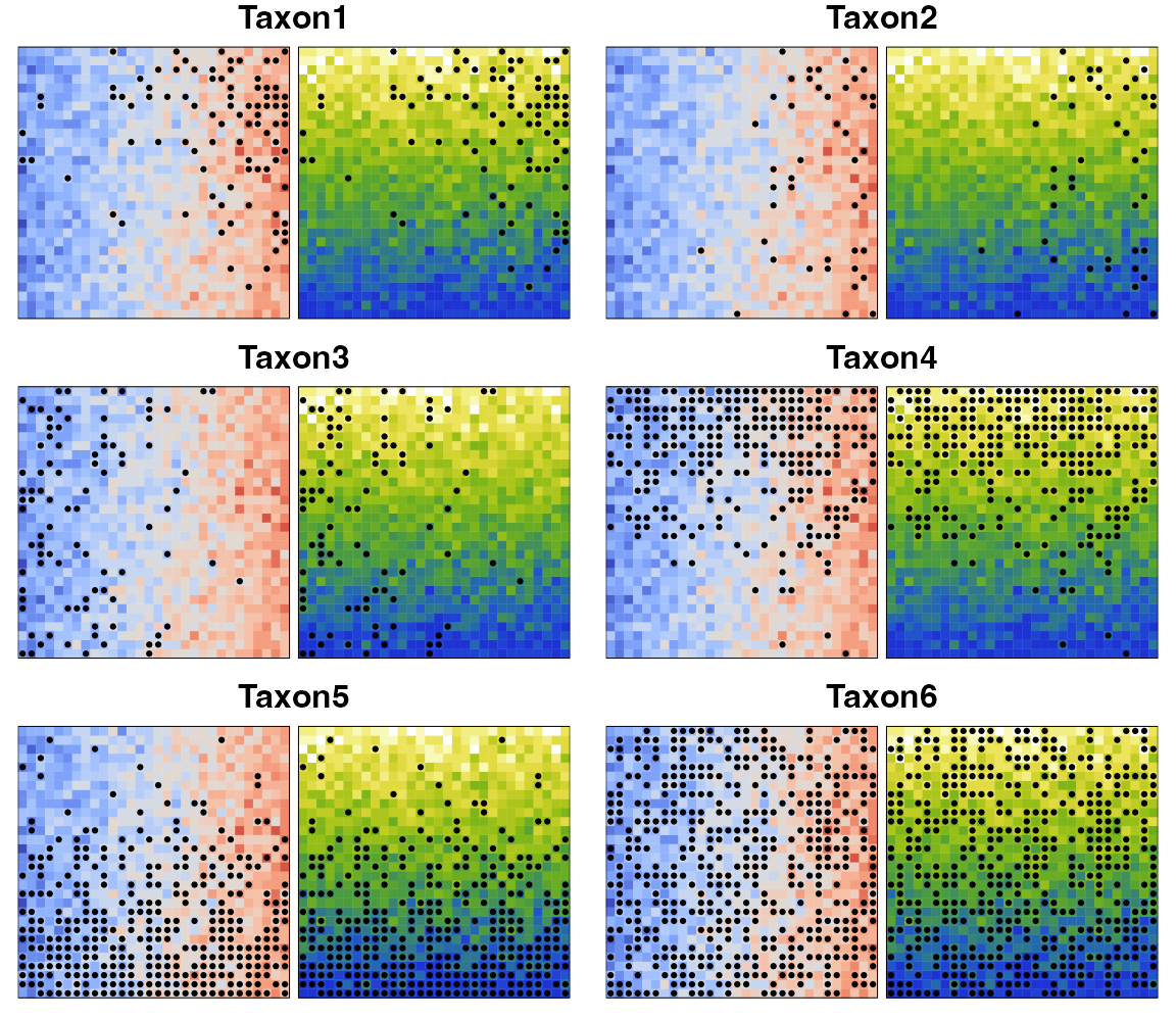
Fig. 2: Distributions of our six taxa of interest (black dots) against the two studied climate gradients.
Finally, we have also created a fossil record composed of 20 samples where the percentages of the different taxa vary (Fig. 3). We selected percentages so that the climate is relatively cold and dry in the first samples, then temperature and precipitation increase. A cold and dry reversal occurs around the middle of the records (samples 11 and 12), and stable humid and warm conditions prevail in the last samples. The top sample also contains a seventh taxon (Taxon7) that doesn’t grow across the study area. It was added to illustrate that crestr can deal with unknown taxa.

Fig. 3: Stratigraphic diagram of the fossil record to be used as the base for temperature and precipitation reconstructions.
The pseudo-data within crestr
The pseudo-data are stored in crestr in different datasets and can be loaded as follow:
The fossil data are contained in crest_ex (“crest
example”). The data frame comprises 20 fossil samples from which the
seven taxa have been identified. The data are already expressed in
percentages.
## the first 6 samples
head(crest_ex)
#>          Age Taxon1 Taxon2 Taxon3 Taxon4 Taxon5 Taxon6 Taxon7
#> Sample_1   1      0      0     45      1     22     32      1
#> Sample_2   2      0      0     50      0     23     27      0
#> Sample_3   3      0      0     49      0     25     26      0
#> Sample_4   4      0      0     37      0     27     36      0
#> Sample_5   5      0      3     36      3     18     40      0
#> Sample_6   6      2      2     25      0     21     50      0

## the structure of the data frame
str(crest_ex)
#> 'data.frame':    20 obs. of  8 variables:
#>  $ Age   : int  1 2 3 4 5 6 7 8 9 10 ...
#>  $ Taxon1: int  0 0 0 0 0 2 3 5 10 15 ...
#>  $ Taxon2: int  0 0 0 0 3 2 5 5 12 8 ...
#>  $ Taxon3: int  45 50 49 37 36 25 18 17 10 12 ...
#>  $ Taxon4: int  1 0 0 0 3 0 0 6 15 14 ...
#>  $ Taxon5: int  22 23 25 27 18 21 21 20 16 13 ...
#>  $ Taxon6: int  32 27 26 36 40 50 53 47 37 38 ...
#>  $ Taxon7: int  1 0 0 0 0 0 0 0 0 0 ...
A proxy-species equivalency (“pse”) table must be provided for each reconstruction. This table is used to associate distinct species to the fossil taxon. For example, in the case of pollen data, this step is used to link all the species producing undifferentiated pollen morphotypes in a single pollen-type. Here, the seven pseudo-taxa are ‘identified’ at the species level so that the table looks like the following:
crest_ex_pse
#>   Level      Family    Genus Species ProxyName
#> 1     3 Randomaceae Randomus  Taxon1    Taxon1
#> 2     3 Randomaceae Randomus  Taxon2    Taxon2
#> 3     3 Randomaceae Randomus  Taxon3    Taxon3
#> 4     3 Randomaceae Randomus  Taxon4    Taxon4
#> 5     3 Randomaceae Randomus  Taxon5    Taxon5
#> 6     3 Randomaceae Randomus  Taxon6    Taxon6
#> 7     3 Randomaceae Randomus  Taxon7    Taxon7
By default, all the identified taxa are used to produce the reconstruction. However, it is sometimes helpful to select a subset of taxa for each variable to improve the signal over noise ratio of the reconstructions. This identification is usually not straightforward and requires some expertise. Here, this information is known because the pseudo-data were generated with apparent sensitivities (see Fig. 2). In crestr, these known sensitivities are expressed in one single table containing 1s (meaning “use this taxon for this variable”) and 0s (meaning “do not use this taxon for this variable”). Based on the description of the sensitivities of the pseudo-taxa (see above), it translates as follow:
crest_ex_selection
#>        bio1 bio12
#> Taxon1    1     1
#> Taxon2    1     0
#> Taxon3    1     0
#> Taxon4    0     1
#> Taxon5    0     1
#> Taxon6    0     0
#> Taxon7    1     1
Note that Taxon7 is indicated with 1s but, as no data are available to calibrate its relationship with climate, these values will later be transformed into “-1”.
The central element of the package: the crestObj
object
In crestr, all the CREST-related data are stored within
a single S3 object of the class crestObj. Most package
functions will take a crestObj as their primary input and
return an updated version of that object. In practice, a
crestObj is a nested list that contains five sub-lists,
each one grouping a specific type of information, such as the
calibration data, the fitted climate responses, or the reconstructions
(Fig. 4). Wrapper functions have been implemented to
manipulate and modify the information contained in a
crestObj, and users are never expected to manually modify
their crestObj– even if it is possible. The five sub-lists
contain the following information:
inputs: contains the input data (e.g. the counts/percentages of the fossil proxy data, the ages of the samples or the names of the fossil taxa).parameters: contains the parameters provided at the different stages of the analysis (e.g. the tailoring of the gbif4crest calibration dataset or the fitting and combination of the PDFs).modelling: contains all the data related to the estimation of the PDFs (e.g. the occurrence data (the ‘distributions’) used to estimate the PDFs, the climate space of the study area, or the PDFs themselves).reconstructions: contains all the results (e.g. best estimates, synthetic error measurements, as well as the full distribution of the reconstruction).misc: contains some additional metadata relative to the reconstruction (e.g. the site location or, most importantly, information related to the proxy-species associated process described in section).
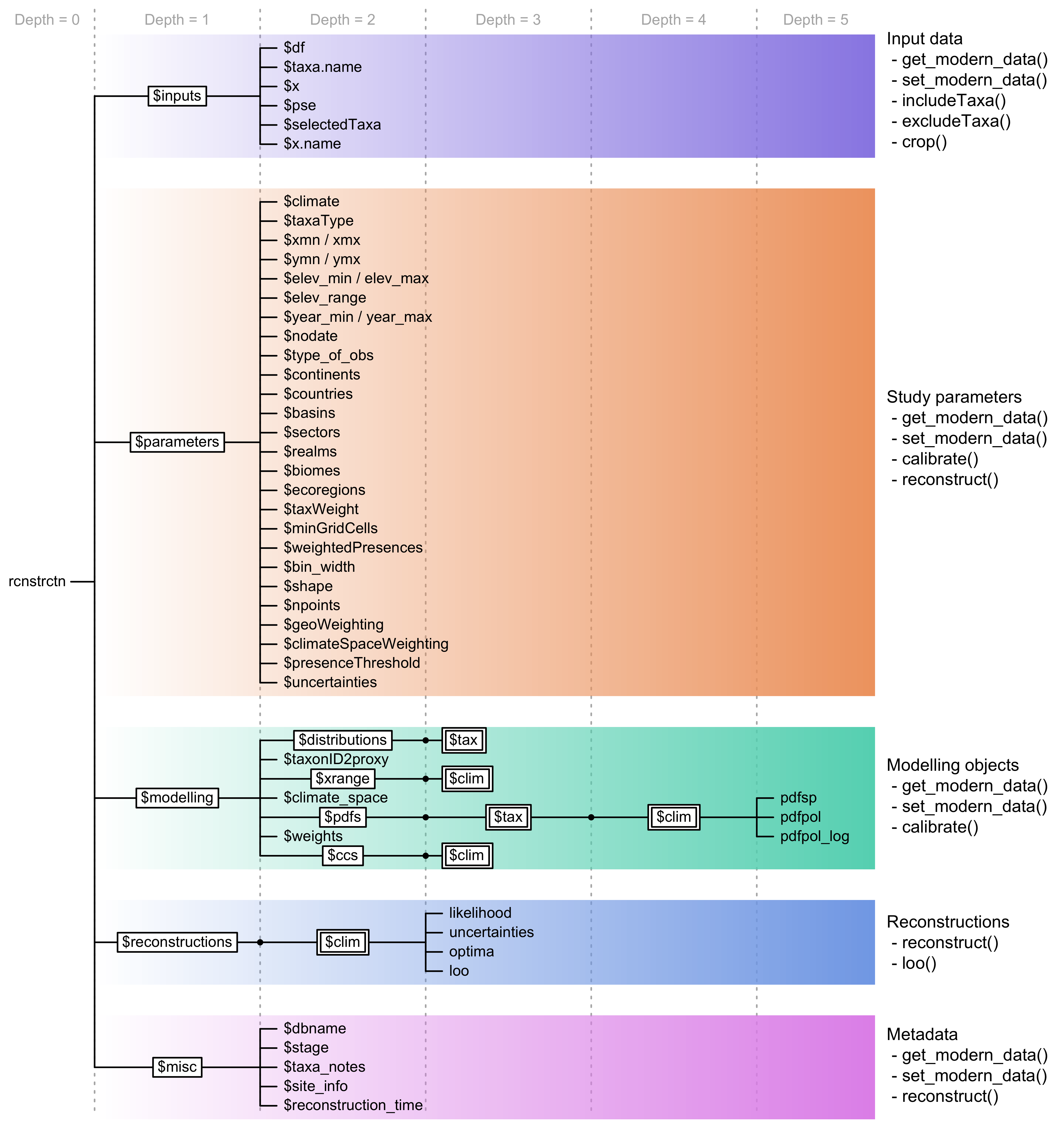
Fig. 4 Structure of a crestObj, here called ‘rcnstrctn’, with the five main sub-lists in colour. For simplicity, lists with many elements (‘tax’ or ‘clim’) are represented with double framed boxes. The unframed terminal nodes on the right-hand side of each branch are simple R objects, such as numbers, strings, vectors or data frames. The names of the functions that modify these obsjects are indicated on the right.
Application: Reconstructions using pseudo-data
Data extraction and calibration
To illustrate the process, we will reconstruct bio1 (mean annual temperature) and bio12 (annual precipitation) from these pseudo data. The complete description of the different parameters is available here.
The first step of any reconstruction is to extract the species
distribution data. This is done with the
crest.get_modern_data() function. This function creates a
nested R object reconstr that contains all the information
that will be updated in the following steps. All the functions from the
package require such an object. For more details, check the
crestObj vignette. We can also verify that the
selectedTaxa table has been modified for Taxon7.
reconstr <- crest.get_modern_data(
                        df = crest_ex, # The fossil data
                   pse = crest_ex_pse, # The proxy-species equivalency table
                         taxaType = 0, # The type of taxa is 0 for the example
              site_info = c(7.5, 7.5), # Coordinates to estimate modern values
             site_name = 'crest-test', # A specific name for the dataset
         climate = c("bio1", "bio12"), # The climate variables to reconstruct
    selectedTaxa = crest_ex_selection, # The taxa to use for each variable
             dbname = "crest_example", # The database to extract the data
                       verbose = FALSE # Print status messages
)
reconstr$inputs$selectedTaxa
#>        bio1 bio12
#> Taxon1    1     1
#> Taxon2    1     0
#> Taxon3    1     0
#> Taxon4    0     1
#> Taxon5    0     1
#> Taxon6    0     0
#> Taxon7   -1    -1
At every step of the process, the content of the crestObj can be checked by printing the object. The information displayed is updated based on the reconstruction step.
print(reconstr, as='data_extracted')
#> *
#> * Summary of the crestObj named ``:
#> *   x Calibration data formatted .. TRUE
#> *   x PDFs fitted ................. FALSE
#> *   x Climate reconstructed ....... FALSE
#> *   x Leave-One-Out analysis ...... FALSE
#> *
#> * The dataset to be reconstructed (`df`) is composed of 20 samples with 7 taxa.
#> * Variables to analyse: bio1, bio12
#> *
#> * The calibration dataset was defined using the following set of parameters:
#> *   x Proxy type ............ Example dataset
#> *   x Longitude ............. [0 - 15]
#> *   x Latitude .............. [0 - 15]
#> *
#> * Of the 7 taxa provided in `df` and `PSE`, 1 cannot be analysed.
#> * (This may be expected, but check `$misc$taxa_notes` for additional details.)
#> *
The next step consists in fitting the PDFs using the crest.calibrate() function. The climate space weighting is selected by default because it is essential to account for the possible heterogeneous distribution of the modern climate when fitting the PDFs. As can be seen in Fig. 5 for temperature, the coldest and warmest values are underrepresented compared to the intermediate values. The correction diminishes the effect of this distribution by upweighting rare values and down-weighting the most abundant ones.
reconstr <- crest.calibrate(
                            reconstr, # A crestObj produced at the last stage
        climateSpaceWeighting = TRUE, # Correct the PDFs for the heteregenous
                                      # distribution of the modern climate space
                bin_width = c(2, 50), # The size of bins used for the correction
    shape = c("normal", "lognormal"), # The shape of the species PDFs
                      verbose = FALSE # Print status messages
)
plot_climateSpace(reconstr)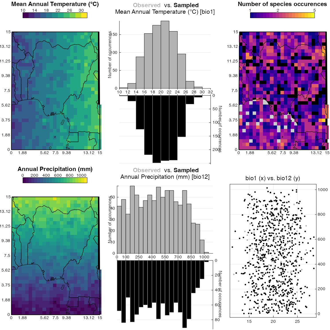
Fig. 5: Distribution of the climate data. The grey histogram represent the abundance of each climate bins in the study area and the black histogram represents how this climate space is sampled by the studied taxa. In a good calibration dataset, the two histograms should be more or less symmetrical. Note: This figure is designed for real data, hence the presence of some African country borders. Just ignore these here.
Other graphical tools can be used to determine the specific sensitivities of each taxon to the selected climate variable. Fig. 6 below represents the characteristic responses of Taxon2 and Taxon7 to bio1. By construction, we know that Taxon2 is sensitive to bio1, while Taxon6 is not. This can be inferred from Fig. 6 by comparing the histograms that represent the proportion of the climate space occupied by each taxon, but also from the width of the PDFs. The PDFs of sensitive taxa are narrower. In the case of Taxon6, its presence in almost every grid cell of the study area indicates that its distribution is not constrained by either bio1 or bio12 at least in this study area. If the spatial scale of the study were changed, some trends in the distribution would ultimately appear.
plot_taxaCharacteristics(reconstr, taxanames='Taxon2', climate='bio1', h0=0.2)
plot_taxaCharacteristics(reconstr, taxanames='Taxon6', climate='bio1', h0=0.2)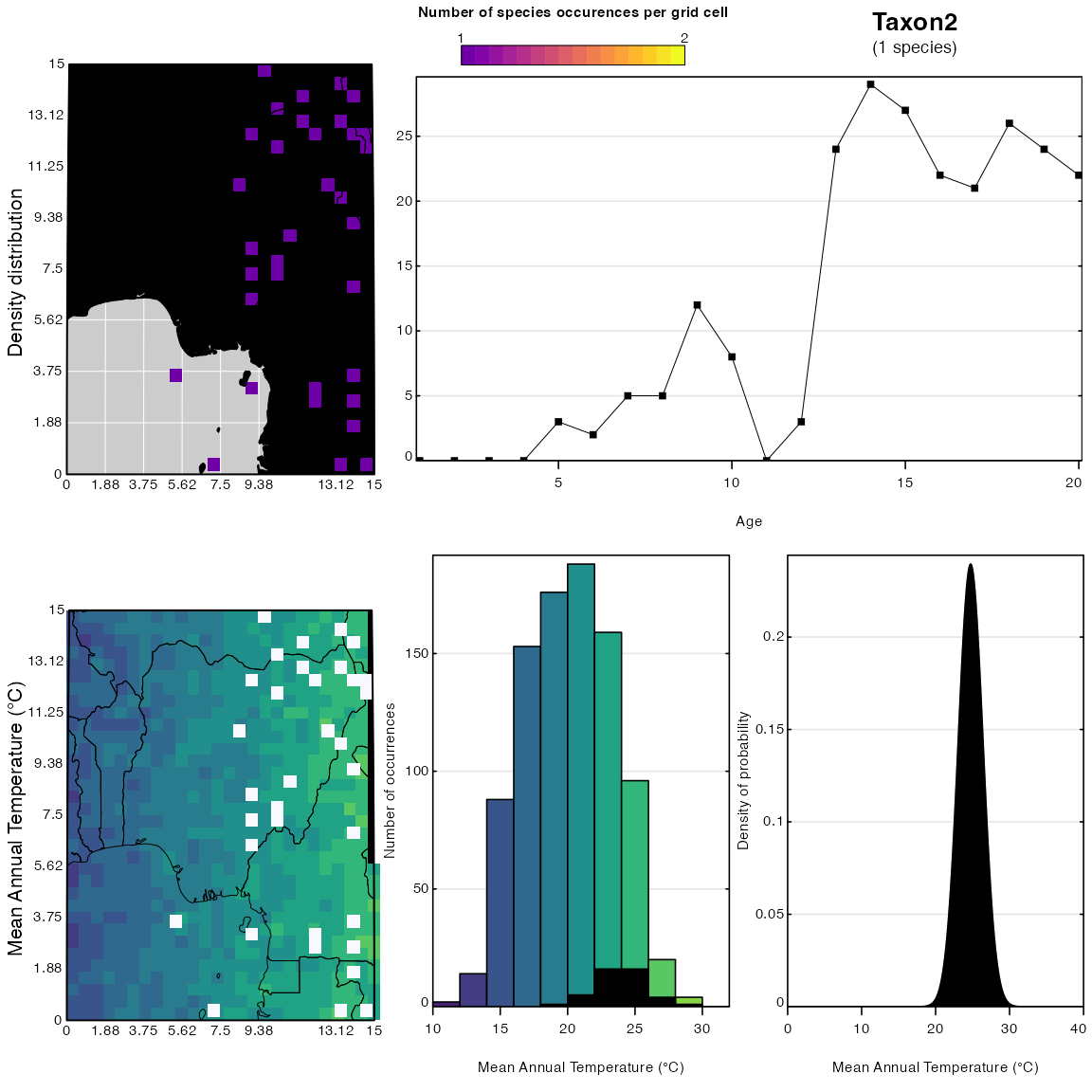
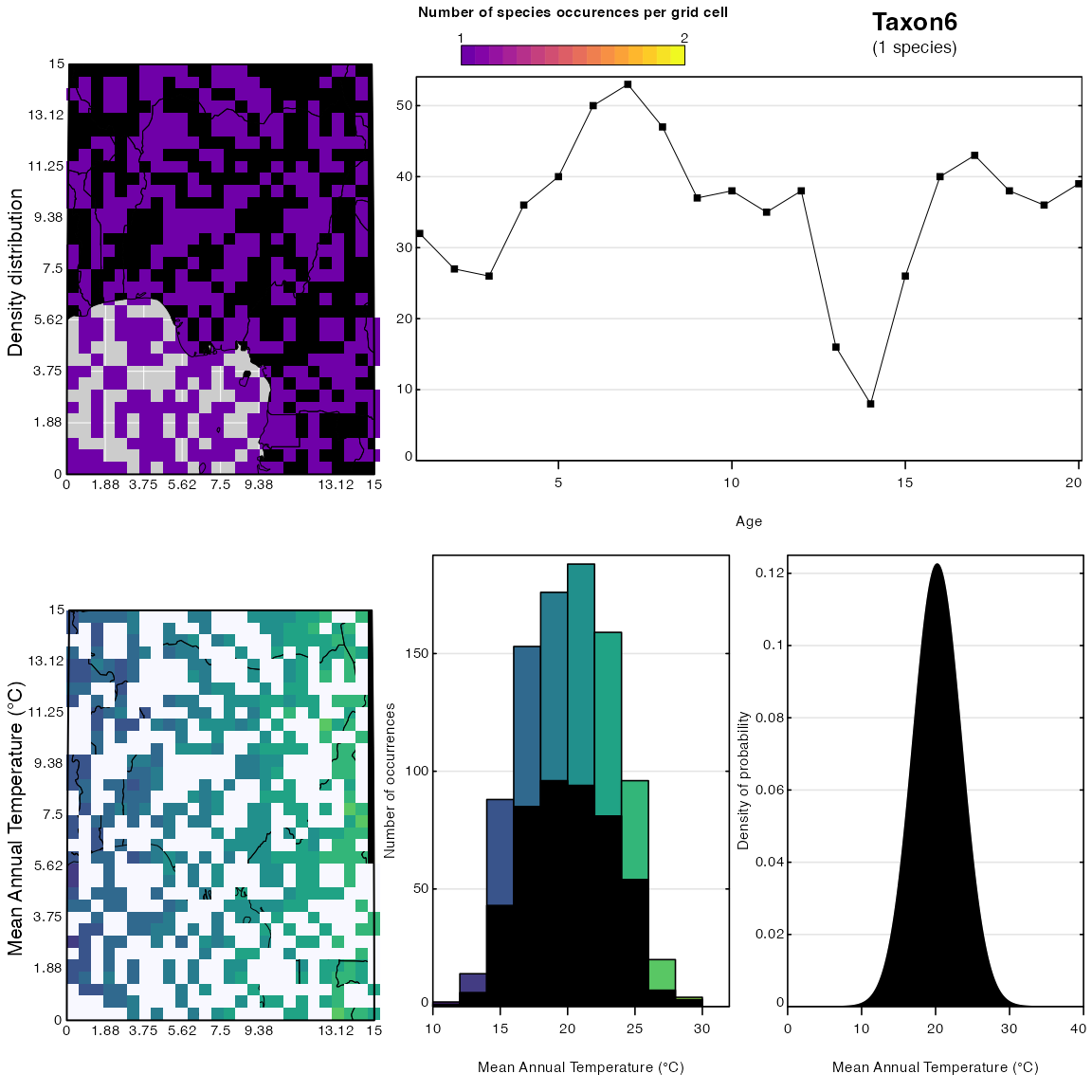
Fig. 6: Distributions and responses of Taxon2 and Taxon6 to bio1. Again, ignore the coastline of Africa on this plot.
Reconstruction and interpretation
The last step of the process is the reconstruction itself, which is
done with the crest.reconstruct() function. The results can be
accessed from reconstr as follow:
reconstr <- crest.reconstruct(
                        reconstr, # A crestObj produced at the previous stage
                  verbose = FALSE # Print status messages
)
names(reconstr)
#> [1] "inputs"          "parameters"      "modelling"       "reconstructions"
#> [5] "misc"

head(reconstr$reconstructions$bio1$optima)
#>   Age   optima     mean
#> 1   1 15.71142 15.69949
#> 2   2 15.71142 15.69949
#> 3   3 15.71142 15.69949
#> 4   4 15.71142 15.69949
#> 5   5 17.31463 17.29054
#> 6   6 18.11623 18.12464

str(reconstr$reconstructions$bio1$optima)
#> 'data.frame':    20 obs. of  3 variables:
#>  $ Age   : num  1 2 3 4 5 6 7 8 9 10 ...
#>  $ optima: num  15.7 15.7 15.7 15.7 17.3 ...
#>  $ mean  : num  15.7 15.7 15.7 15.7 17.3 ...

signif(reconstr$reconstructions$bio1$likelihood[1:6, 1:6], 3)
#>          [,1]     [,2]     [,3]     [,4]     [,5]     [,6]
#> [1,] 0.00e+00 8.02e-02 1.60e-01 2.40e-01 3.21e-01 4.01e-01
#> [2,] 8.41e-15 1.15e-14 1.57e-14 2.14e-14 2.92e-14 3.97e-14
#> [3,] 8.41e-15 1.15e-14 1.57e-14 2.14e-14 2.92e-14 3.97e-14
#> [4,] 8.41e-15 1.15e-14 1.57e-14 2.14e-14 2.92e-14 3.97e-14
#> [5,] 8.41e-15 1.15e-14 1.57e-14 2.14e-14 2.92e-14 3.97e-14
#> [6,] 1.45e-18 2.09e-18 3.01e-18 4.32e-18 6.19e-18 8.86e-18

str(reconstr$reconstructions$bio1$likelihood)
#>  num [1:21, 1:500] 0.00 8.41e-15 8.41e-15 8.41e-15 8.41e-15 ...

print(reconstr, as='climate_reconstructed')
#> *
#> * Summary of the crestObj named ``:
#> *   x Calibration data formatted .. TRUE
#> *   x PDFs fitted ................. TRUE
#> *   x Climate reconstructed ....... TRUE
#> *   x Leave-One-Out analysis ...... FALSE
#> *
#> * The dataset to be reconstructed (`df`) is composed of 20 samples with 7 taxa.
#> * Variables to analyse: bio1, bio12
#> *
#> * The calibration dataset was defined using the following set of parameters:
#> *   x Proxy type ............ Example dataset
#> *   x Longitude ............. [0 - 15]
#> *   x Latitude .............. [0 - 15]
#> *
#> * The PDFs were fitted using the following set of parameters:
#> *   x Minimum distinct of distinct occurences .. 20
#> *   x Weighted occurence data .................. FALSE
#> *   x Number of points to fit the PDFs ......... 500
#> *   x Geographical weighting ................... TRUE
#> *       Using bins of width .................... bio1: 2
#> *       ________________________________________ bio12: 50
#> *   x Weighting of the climate space ........... TRUE
#> *       Using a linear correction
#> *   x Restriction to climate with observations . FALSE
#> *   x Shape of the PDFs ........................ bio1: normal
#> *     __________________________________________ bio12: lognormal
#> *
#> * Of the 7 taxa provided in `df` and `PSE`, 1 cannot be analysed.
#> * (This may be expected, but check `$misc$taxa_notes` for additional details.)
#> *
#> * The reconstructions were performed with the following set of parameters:
#> *   x Minimum presence value .................. 0
#> *   x Weighting of the taxa ................... normalisation
#> *   x Calculated uncertainties ................ 0.5, 0.95
#> *   x Number of taxa selected to reconstruct .. bio1: 3
#> *     ----------------------------------------- bio12: 3
#> *
The results can also be visualised in different forms using the plot function (Fig. 7). As per the design, the first samples are rather cold and dry, while the last ones are relatively warm and humid. A cold and dry event interrupted the transition between the two states.
plot(reconstr, climate = 'bio1')
plot(reconstr, climate = 'bio12', simplify=TRUE,
        uncertainties=c(0.4, 0.6, 0.8), as.anomaly=TRUE)
#> Warning in plot.crestObj(reconstr, climate = "bio12", simplify = TRUE,
#> uncertainties = c(0.4, : No values available to calculate anomalies. Provide
#> coordinates to crest.get_modern_data() to allow crestr to extract the local
#> conditions, or assign values using 'anomaly.base = c(val1, val2, ...)' in the
#> plot function.'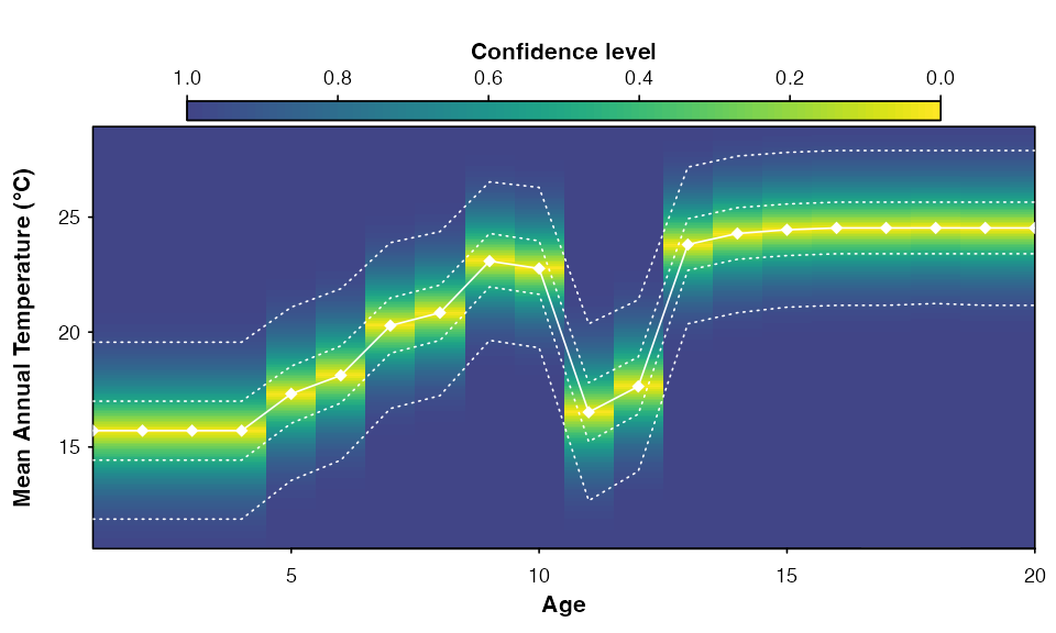
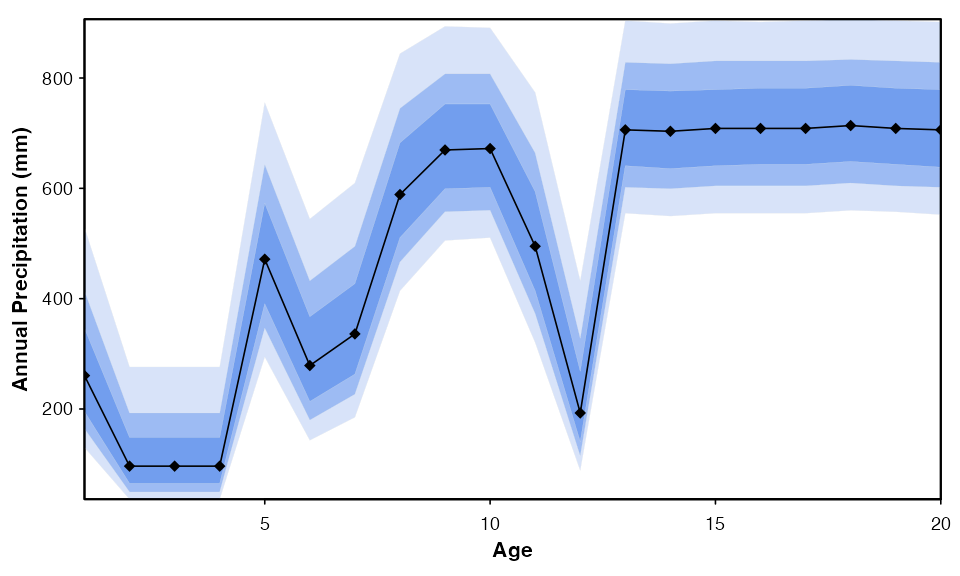
Fig. 7: (top) Reconstruction of mean annual temperature with the full distribution of the uncertainties. (bottom) Reconstruction of annual precipitation using the simplified visualisation option. In both cases, different levels of uncertainties can be provided.
Interpretations can be refined using the built-in ‘leave-one-out’ (loo) approach. The loo approach iteratively removes one taxon at a time and measures the impact removing that taxon had on the ‘true’ reconstruction. The results can be plotted as a stratigraphic diagram.
reconstr <- loo(reconstr)
plot_loo(reconstr, climate = 'bio1')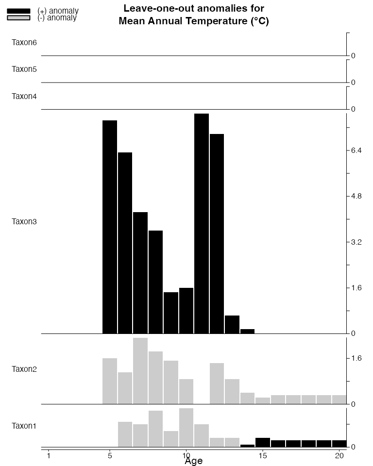
Fig. 8: Leave-One-Out diagram for the reconstructions of bio1.
Exporting the results
If satisfying, the results can be directly exported from the R
environment in individual spreadsheets for each variable (or CSV files).
The reconstruct object is exported as an RData file to
simplify future data reuse. In the following lines of code, replace
‘tempdir()’ with the location where the files should be saved.
export(reconstr, loc=tempdir(), dataname='crest-test')
list.files(file.path(tempdir(), 'crest-test'))
#> [1] "bio1"             "bio12"            "crest-test.RData"
References
[1] Chevalier, M., 2022. crestr an R package to perform probabilistic climate reconstructions from palaeoecological datasets. Clim. Past. doi:10.5194/cp-18-821-2022.
[2] Chevalier, M., Chase, B.M., Quick, L.J., Dupont, L.M. and Johnson, T.C., 2021. Temperature change in subtropical southeastern Africa during the past 790,000 yr. Geology 49, 71–75. 10.1130/G47841.1.
[3] Chevalier, M., Chase, B.M., 2015. Southeast African records reveal a coherent shift from high- to low-latitude forcing mechanisms along the east African margin across last glacial–interglacial transition. Quat. Sci. Rev. 125, 117–130. doi:10.1016/j.quascirev.2015.07.009.
[4] Quick, L.J., Chase, B.M., Carr, A.S., Chevalier, M., Grobler, B.A. and Meadows, M.E., 2021, A 25,000 year record of climate and vegetation change from the southwestern Cape coast, South Africa. Quaternary Research, pp. 1–18. 10.1017/qua.2021.31.
[5] Chevalier, M., Chase, B. M., Quick, L. J. and Scott, L.: An atlas of southern African pollen types and their climatic affinities, in Palaeoecology of Africa, vol. 35, pp. 239–258, CRC Press, London., 2021. 10.1201/9781003162766-15.